Smooth markers

Raw animated 3D markers used in motion analysis or rigid body animation have some level of noise due mostly to digitizing or tracking errors. This tutorial will show you how to smooth the trajectories of tracked markers over time to remove this noise and create smooth plotted trajectories and animations. The uninterrupted block of code can be found at the end of this tutorial.

Preliminary steps

Make sure that you have R installed on your system (you can find R installation instructions here).Next, install the beta version (v1.0) of the R package "matools" (not yet on CRAN). You can do this by downloading this folder (< 1MB), unzipping the contents, and then running the commands below to install the package.

# Set the path to where the package was unzipped (customize this to your system)
pkg_path <- '/Users/aaron/Downloads/matools-master'

# Run the install.packages function on the matools-master folder
install.packages('/Users/aaron/Downloads/matools-master', repos=NULL, type='source')

Alternatively, you can install "matools" using the function install_github, from the R package devtools.

# Load the devtools package (once installed)
library(devtools)

# Install the version of matools currently on github
install_github('aaronolsen/matools')

Once the package is installed, use the library function to load the package.

# Load the matools package
library(matools)

Non-adaptive smoothing

To smooth a set of 3D coordinates you'll need an array of coordinates (in which the third dimension is the position of each coordinate over time). This can be a '3D Points' file exported from XMALab, for example.

You can try out the code in this tutorial using this unsmoothed 3D marker coordinates file. This file contains the 3D coordinates of radiopaque markers implanted in a channel catfish eating a worm, captured using XROMM and tracked using XMALab. This tutorial file also contains extra metadata associated with the trial (e.g. calibration, frame number, etc.), though we are just interested in the marker coordinates at this point. Download the file and move it to your current R working directory and then read the animated coordinates from the file using the readMotion function ("matools" package).

# Read unsmoothed motion
read_motion <- readMotion('Cat01 Trial09 marker motion raw.csv')

The readMotion function returns a 'motion' object containing the marker coordinates ($xyz) and the additional metadata. You can preview the contents of this object using the print function. The output of the print command shows you the number of iterations (i.e. "time points") in the motion object (here, 1819), the names of the "xyz" (i.e. marker) coordinates, and all of the metadata columns ("calibration", "frame", etc.).

# See what is contained in the motion object (optional)
print(read_motion)

Next input this motion object into smoothMotion. We'll start with the simplest type of call to smoothMotion in which a single smoothing parameter is applied across the entire time sequence (non-adaptive smoothing). Include a file path where you would like to save a PDF diagnostic plot using the plot.diag parameter; the diagnostic plot is essential to making sure you have selected an appropriate degree of smoothing.

# Smooth points in the motion object
smooth_motion <- smoothMotion(read_motion, plot.diag='Cat01 Trial09 marker motion raw.pdf')

Note that smoothMotion can also accept a simple 3D point array instead of a motion object. For example, this also works:

# smoothMotion also accepts a simple 3D point array
smooth_motion <- smoothMotion(read_motion$xyz, plot.diag='Cat01 Trial09 marker motion raw.pdf')

The smoothMotion function smoothes each dimension of each marker using the loess function (R "stats" package). The loess function uses polynomial fitting with degree of smoothing controlled by the parameter span. The degree of smoothing with loess depends on the length of the time sequence so span must be adjusted as the time sequence increases or decreases. The smoothMotion function performs this adjustment for you but you can still specify the degree of smoothing using the span.factor parameter. The default value for this parameter is 18; this is a value that I have found to work well using different motion datasets but you may need to adjust this value.

Take a look at the diagnostic plot output by smoothMotion. For each marker, smoothMotion creates two plots side-by-side:

1. the raw and smoothed x-, y-, and z-values over time (mean-centered so they fit nicely in the same plot)
2. the deviation of the smoothed values from the raw values over time

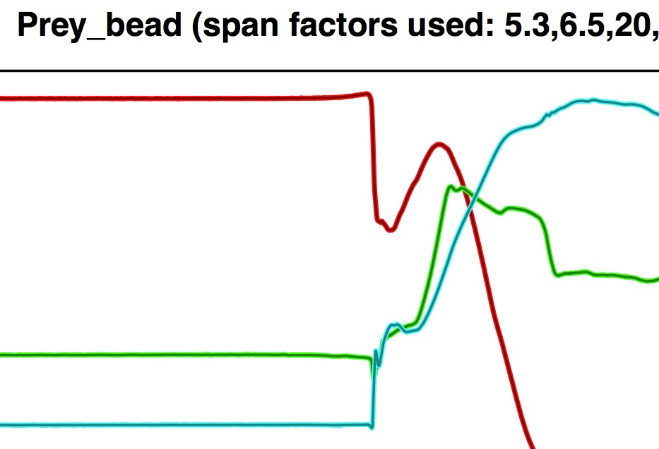
Note that since this tutorial file has 38 marker coordinates this is a fairly "tall" PDF. Below is a close-up of the row corresponding to the "prey bead" (a marker implanted into the prey item).

Diagnostic plots created by smoothMotion for each marker showing the raw and smoothed values (left) and the deviation of the smoothed from the raw values (right).

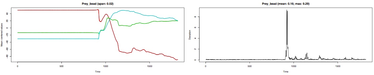
If you zoom into the left plot of the PDF you can see the smoothed xyz-values (darker, thinner line) superimposed on the raw xyz-values.

Close-up of smoothed xyz coordinates (darker) superimposed on raw (lighter) coordinates. Smoothed values miss some consistent trends in the raw values.

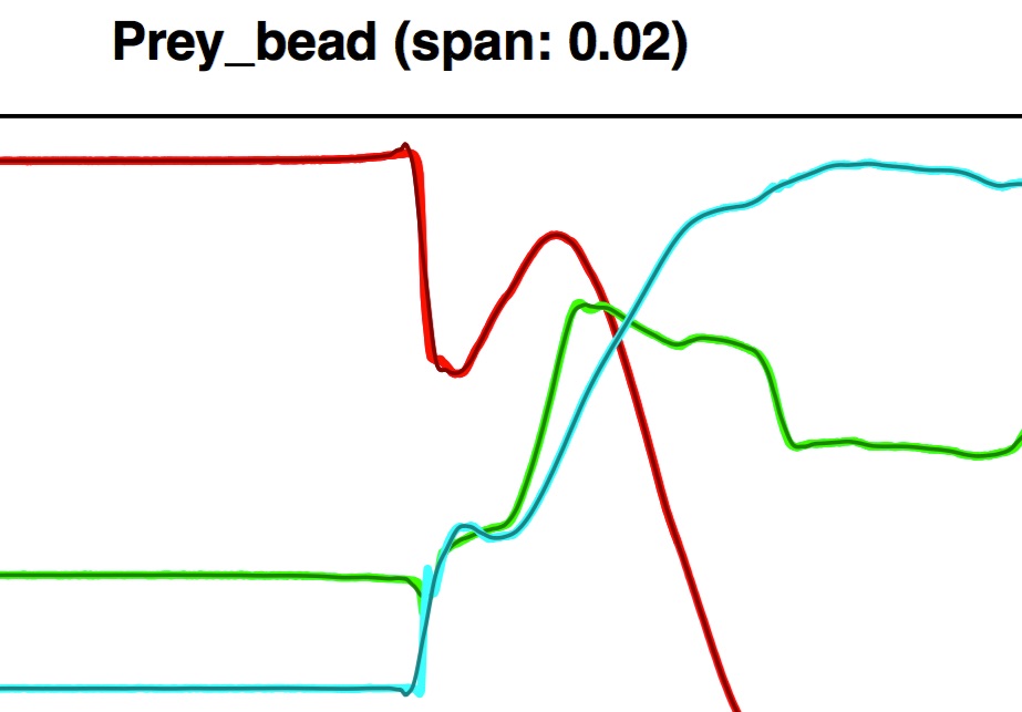
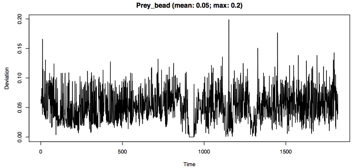
In some areas the smoothing looks pretty good but the time at which the prey marker suddenly starts moving (i.e. accelerates) and then starts moving more slowly (i.e. decelerates) there is a mismatch between the raw and unsmoothed coordinates. This is especially evident when looking at the deviation of the smoothed coordinates over time.

A close-up of deviation of smoothed coordinates from raw coordinates. Broad peaks (more than 1-2 frames) suggest excessive smoothing.

In the deviation plot, sharp peaks (1-2 frames only) usually indicate tracking errors (e.g. the wrong bead has been identified) while broad peaks (more than 1-2 frames) usually indicate excessive smoothing. The above close-up of the deviation plots has broad peaks meaning that for some frames the smoothing that we have chosen is too strong. One option is to decrease the degree of smoothing (by decreasing the span.factor parameter).

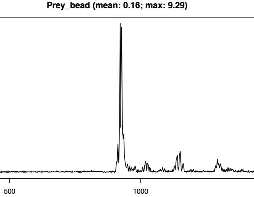
# Decrease the degree of smoothing by decreasing span.factor (default is 18)
smooth_motion <- smoothMotion(read_motion$xyz, plot.diag='Cat01 Trial09 marker motion raw low.pdf', 
	span.factor=2)

This improves the overlap between the raw and smoothed coordinates a bit but an inherent problem here is that the smoothing is being applied over regions with little to no motion and regions with rapid changes in speed.

A span.factor of 2 still doesn't quite capture the motion of the prey marker.

In addition, choosing a lower degree of smoothing might help with one marker but may increase the noise elsewhere. What we need is to apply the smoothing over regions with similar velocity profiles and "adapt" the degree of smoothing depending on the characteristics of each region. This is covered in the next section on adaptive smoothing.

Adaptive smoothing

Adaptive smoothing allows the smoothing parameter to vary over time to better match the noise-to-signal characteristics of a particular region of signal and applies the smoothing to a localized region of values. The smoothMotion function performs adaptive smoothing by applying a single (high) smoothing parameter, finding the deviation of the raw values from the smoothed values, and separating the raw values into bins based on a sliding window of mean deviations. The raw values are then smoothed using different values for each bin. In this way raw values that deviate least from high smoothing keep a high degree of smoothing while raw values that deviate the most from high smoothing are smoothed at a lower degree so that signal is not "smoothed out".

The user specifies the number of bins, the deviation values that divide the bins, and the smoothing parameter applied to each bin. Finding the right values for your data may take some experimentation, trying out different values and examining the diagnostic plots. But in my experience once you find a set of parameters that are suitable for one trial you can apply these parameters to all of your trials.

Set the number of bins, the deviation values that separate the bins, and the smoothing parameter applied to each bin using the span.factor and smooth.bins parameters. Instead of using a single value, use span.factor to input a vector of smoothing values, one for each bin. These should be listed in decreasing order (the highest degree of smoothing first). The following values work well for the tutorial trial.

# Set smoothing strength (higher = more smoothing)
span.factor <- c(33, 20, 6.5, 5.3)

Then set smooth.bins to the deviation values that define the "boundaries" between consecutive bins. This vector will have one more value than the number of bins (the first two values define the boundaries of the first bin, the second and third values define the boundaries of the second bin, etc.). Note that if you want all your raw values smoothed the last value should be the maximum mean deviation that you expect; you can just choose a very large value (e.g. 1000). You may want to not apply any smoothing to values that deviate the most from high smoothing (e.g. rapidly changing values); in this case you can set this lower so that those values do not fall in any bin. For the tutorial trial we are using 4 bins so smooth.bins has 5 values; the following values should work well.

# Set the deviation values separating bins
smooth.bins <- c(0, 0.05, 0.11, 0.30, 1000)

Now call smoothMotion as before but with the added parameters: span.factor, smooth.bins, and bin.replace.min. The bin.replace.min is the minimum number of frames that each bin should have.

# Smooth points
smooth_motion <- smoothMotion(read_motion, span.factor=span.factor, 
	smooth.bins=smooth.bins, plot.diag='Cat01 Trial09 marker motion raw adaptive.pdf', 
	bin.replace.min=10, adaptive=TRUE)

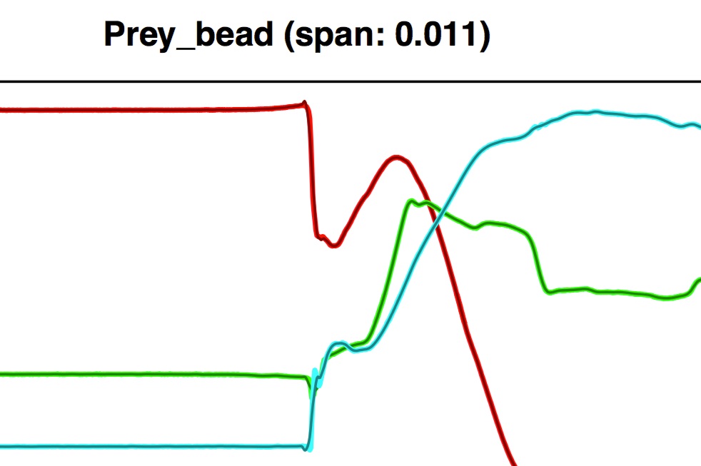
When using adaptive smoothing an additional plot is added to diagnostic plot file (shown below for the prey marker).

The bins assigned to each region indicated by "flat-top" lines, based on an initial rolling mean deviation from high smoothing.

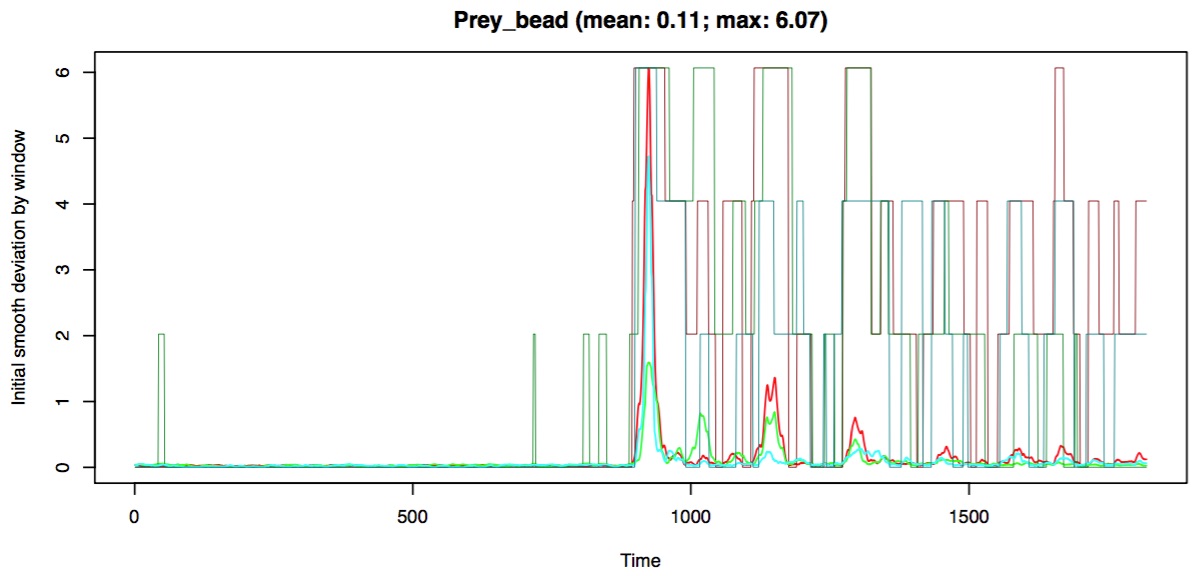
This plot shows you the bin assignments for each dimension (x,y,z) as a series of "flat-top" lines. No visible flat-top line indicates those values were placed in the first bin (highest smoothing) while the tallest flat-top line indicates those values were placed in the last bin (least smoothing). These flat-top lines are superimposed on the rolling mean deviation of the values from an initial smoothing (using the highest smoothing parameter specified by the user), indicated on the y-axis. Note that the height of the flat-top lines does not correspond to the y-axis values and that each color (red, green, blue) corresponds to each dimension (x, y, z, respectively).

Using adaptive smoothing the deviation between raw and smoothed values for the prey marker now looks uniform across the trial. There is a small region just before frame 1000 where the deviation is 0; this indicates that there was no smoothing performed in that region (i.e. the raw values are equal to smoothed values). This can happen when a bin is so small and the values so variable that the loess function fails.

The deviation between raw and smoothed values for the prey marker after adaptive smoothing.

Here this is ideal because this region corresponds to place on the trajectory curve when the prey goes from not moving to sudden accelerations in different directions; it's not really appropriate to apply smoothing to this region of the prey's trajectory. Visual inspection of the coordinate trajectory plot also shows that adaptive smoothing has produced nice overlap between the smoothed values and the raw values for the prey marker.

The smoothed and raw coordinate values match nicely when adaptive smoothing is applied.

Saving the results

The last step is to save these results. If you input a motion file, the output will be a motion object with all the original metadata. You can save the motion object using using writeMotion.

# Save smoothed coordinates as motion object
writeMotion(x=smooth_motion, file='Cat01 Trial09 marker motion smoothed.csv')

If you input an array of 3D points then the output will also be an array of 3D points that you can save using the writeLandmarks function.

# Save smoothed coordinates (if you input a 3D array)
writeLandmarks(x=smooth_motion, file='Cat01 Trial09 marker motion smoothed.csv')