Rigid body animation

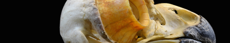
To create a marker-based animation of rigid bodies one needs two types of data. The first is a body either with markers fixed to the outside of the body (if using light cameras) or markers embedded inside of the body (if using X-ray cameras). The rigid bodies can be simple geometric shapes representing rigid elements or full surface meshes, constructed from surface or CT scans such as below.

Four rigid skeletal elements from a channel catfish skull with embedded markers (small metal beads). The surface meshes were created from a CT scan.

The second type of data is the motion of those markers over time.

The corresponding motions of each of the markers in the previous image (colored lines) as measured from stereo X-ray video, with positions at four particular time points indicated by spheres.

These two data types can then be combined (or "unified") to create a rigid body animation. At each time point, the marker motion coordinates are used to set the position and orientation of each rigid body (together these are known as the "pose" of a body).

After unification the rigid bodies (meshes from a CT scan) are animated using the marker motions. Four time points are shown from an animation of the channel catfish skull, collected from stereo X-ray video.

Preliminary steps

Make sure that you have R installed on your system (you can find R installation instructions here).Next, install the beta version (v1.0) of the R package "matools" (not yet on CRAN). You can do this by downloading this folder (< 1MB), unzipping the contents, and then running the commands below to install the package.

# Set the path to where the package was unzipped (customize this to your system)
pkg_path <- '/Users/aaron/Downloads/matools-master'

# Run the install.packages function on the matools-master folder
install.packages('/Users/aaron/Downloads/matools-master', repos=NULL, type='source')

Alternatively, you can install "matools" using the function install_github, from the R package devtools.

# Load the devtools package (once installed)
library(devtools)

# Install the version of matools currently on github
install_github('aaronolsen/matools')

Once the package is installed, use the library function to load the package.

# Load the matools package
library(matools)

Unification

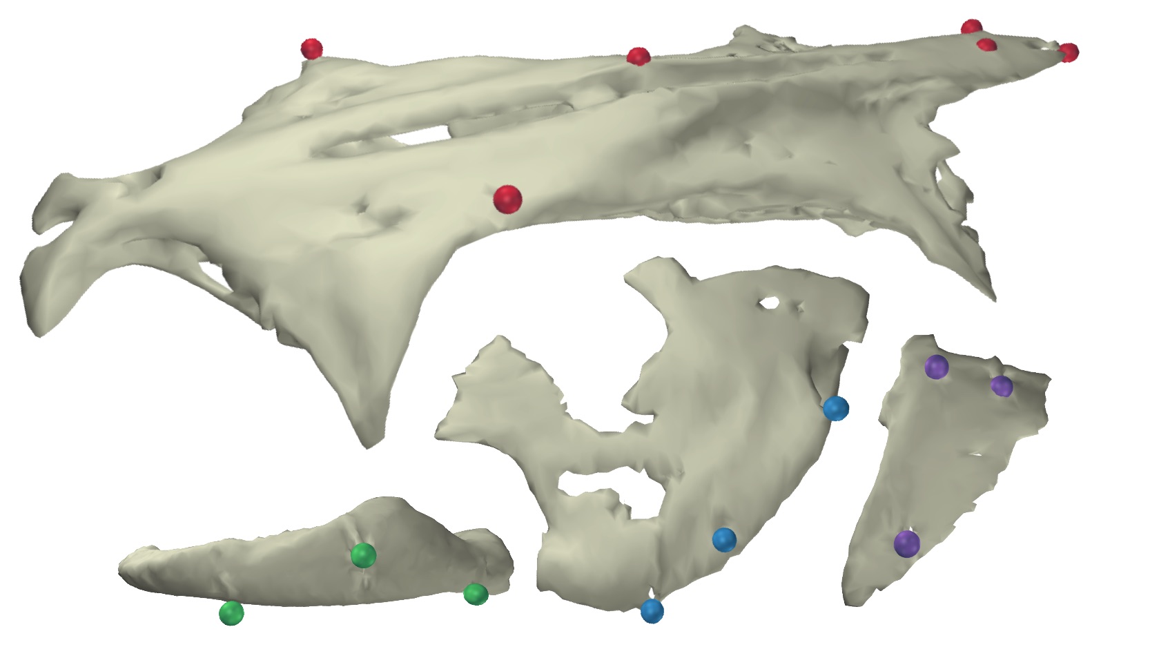
For unification you'll first need a set of 3D marker coordinates, either on the surface of or embedded within a marked body or bodies. For example, these can be the 3D marker coordinates from a CT or surface scan of the body. Since these are not animated they take the form of a simple matrix. For this tutorial, you can use this landmark coordinates file (as a .csv), containing the markers embedded in the channel catfish skull shown in the introduction above. After downloading the file and moving it to your current R working directory, you can read the landmarks using readLandmarks.

## Unification (solving for body transformations)
# Read landmark coordinates
landmarks <- readLandmarks('Cat01 landmarks.csv')

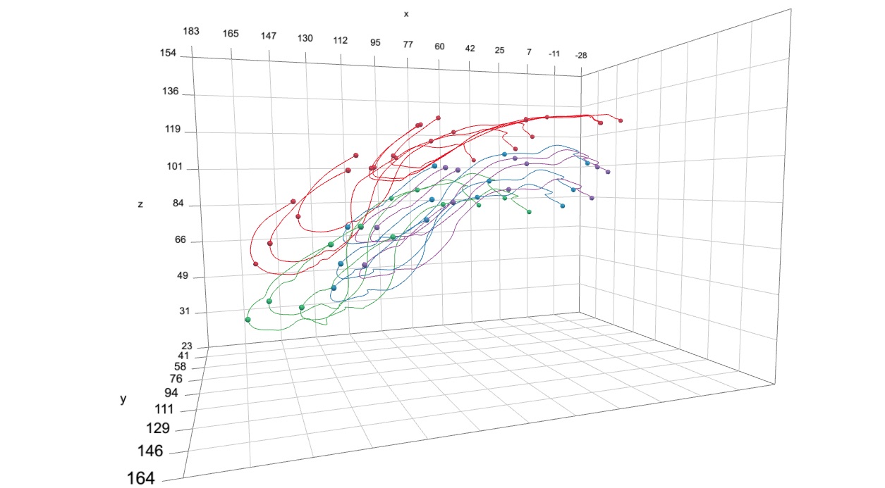
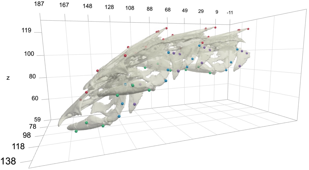
Next you'll need the positions of these same markers over time in the form of an array (in which the third dimension is each frame or time point). For example, these can be markers tracked and reconstructed using XMALab and exported as a '3D Points' file. To produce a smooth animation you can first smooth the marker trajectories. For this tutorial, you can use this smoothed 3D marker coordinates file, which was created in the marker smoothing tutorial. This file contains the 3D coordinates of radiopaque markers implanted in a channel catfish, collected using XROMM and tracked using XMALab. After downloading the file and moving it to your current R working directory, you can read this file using readMotion.

# Read smoothed marker motion
read_motion <- readMotion('Cat01 Trial09 marker motion smoothed.csv')

It is essential that both the landmark and motion coordinates of the markers be at the same scaling. So if your motion capture system and scanning software operate on different units, you'll need to convert one of the two so that the units are the same. The tutorial datasets used here are both already scaled to the same units (mm). If you need to change the scaling for your data you can simply multiply read_motion$xyz by a factor like below.

# Marker motion coordinates can be scaled like this (not needed for tutorial datasets)
read_motion$xyz <- read_motion$xyz * 10

Lastly, it is necessary to specify which markers will be used in animating each rigid body. This is done using a list object, in which the names of each list item correspond to the name of each body and the values of each item are the markers to be used for that particular body. When listing multiple markers, they should be in a list element named 'align'. For example, the list below can be used with the tutorial landmark and motion files.

# Specify which bodies to animate and which markers to use for each body
unify.spec <- list(
	'Neurocranium'=list('align'=c('Neurocranium_bead_cau', 'Neurocranium_bead_cau_e1', 
		'Neurocranium_bead_cau_e2', 'Neurocranium_bead_cra_L', 'Neurocranium_bead_cra_R', 
		'Neurocranium_bead_mid')),
	'SuspensoriumL'=list('align'=c('SuspensoriumL_bead_dor', 'SuspensoriumL_bead_mid', 
		'SuspensoriumL_bead_ven')),
	'LowerJawL'=list('align'=c('LowerJawL_bead_cau', 'LowerJawL_bead_cra', 'LowerJawL_bead_mid')),
	'OperculumL'=list('align'=c('OperculumL_bead_cau_dor', 'OperculumL_bead_cra_dor', 
		'OperculumL_bead_ven'))
)

Note that the neurocranium has six markers while the rest of the elements all have three markers. To solve for the pose of a body in 3D using only markers, the body must have at least three markers that are not co-linear (all in a line). Even then, more than three markers is preferable to minimize error. Further along this tutorial will explain how to animate a body with fewer than three markers, however this requires additional information or requires making simplifying assumptions.

It's now possible to call the unifyMotion function. There are three additional parameters to note at this point. The first is print.progress, which if TRUE will print out exactly what unifyMotion is doing step by step (default is FALSE). The print.progress.iter parameter is the iteration (or iterations) for which the step-by-step progress will be printed (default is 1). Note that the errors that are printed to the console as a part of print.progress are only the errors for that particular iteration, not the entire sequence. Lastly, the plot.diag can be used to create a plot showing the unification errors (how well the corresponding marker sets align with each other) over the entire animation sequence (default is NULL). The code below will create a pdf named 'Unification errors.pdf'.

# Unify landmarks and motion to create an animation
unify_motion <- unifyMotion(read_motion, xyz.mat=landmarks, unify.spec=unify.spec, 
	print.progress=TRUE, print.progress.iter=1, plot.diag='Unification errors.pdf')

The unifyMotion function returns two objects, a 'motion' object (unify_motion$motion) and an error matrix (unify_motion$error). A first thing to do after running unifyMotion$motion is to check the unification errors using the print command.

# Check the unification errors
print(unify_motion$error)

This will print the error for each body for the first five iterations and then summary statistics for all iterations (min, max, and mean).

     $LowerJawL $Neurocranium $OperculumL $SuspensoriumL
1    0.02293696    0.09415792  0.05953781     0.09642377
2    0.01589944    0.09062001  0.05473783     0.09440632
3    0.01623216    0.08753566  0.05061602     0.09254273
4    0.01828475    0.08490102  0.04720247     0.09081870
5    0.01918041    0.08268930  0.04437062     0.08927868
... and 1814 more rows
     $LowerJawL $Neurocranium $OperculumL $SuspensoriumL
min     0.00665       0.03968     0.00129        0.01347
max     0.28014       0.19107     0.12133        0.31113
mean    0.05060       0.09436     0.03758        0.09758

These errors are the error after aligning the marker landmarks with the markers from the motion data. If a body were perfectly rigid (i.e. no bending, stretching, etc.) and if the marker motions were collected with perfect accuracy the unification errors would be zero. However, deformation of the body and errors in motion capture will inevitably lead to some unification errors. In this case the errors do not exceed 0.31 mm (310 microns), which amounts to 1% or less of the total length of the bodies we are animating.

Of course another next step after unification is to create an actual animation to visualize the motion of the bodies. The key piece to creating an animation is returned from unifyMotion as a part of the 'motion' object, specifically unify_motion$motion$tmat, which is an array containing a transformation matrix for each element at each iteration. The next section will show how to use this 'tmat' object and the R package svgViewR to create an animation.

Creating an animation

To create a rigid body animation in R, we'll use the R package svgViewR. This package creates interactive animations as standalone html files using the threejs javascript library.

Creating an svgViewR visualization uses a similar approach to plotting to pdf or image files in R. Start by declaring a new file using the svg.new function, including where you would like to save the file and the name you would like to give it.

## Create an animation
# Declare a new visualization file
svg.new(file='Rigid body animation.html', mode='webgl')

Next add the surface models for each body and markers to the "scene". If you're using the tutorial files you can download the surface mesh files for each of the skeletal elements as a compressed folder here.

The easiest way to add each element is to loop through the names of the unify parameters list unify.spec. To add a surface mesh to the scene use the svg.mesh function (note that currently this only works with OBJ surface models). To create the animation we are going to transform these surface models using the transformation matrices output from unifyMotion. But in order to known which model is which we have to specify a name for each mesh. This is done using the name parameter in the svg.mesh function.

# For each body in unify.spec names
for(body_name in names(unify.spec)){

	# Add surface mesh (OBJ) of body
	svg.mesh(file=paste0('meshes/Cat 01 ', body_name, '.obj'), name=body_name)
	
	# Find markers corresponding to body using regular expression matching
	markers_match <- grepl(paste0('^', body_name, '_'), dimnames(read_motion$xyz)[[1]])

	# Get marker names from first dimension of xyz motion coordinates
	body_markers <- dimnames(read_motion$xyz)[[1]][markers_match]

	# Plot markers from motion capture (already animated)
	svg.spheres(x=read_motion$xyz[body_markers,,], col='yellow')

	# Plot markers as landmarks (static matrix to be transformed)
	svg.spheres(x=landmarks[body_markers,], col='gray', name=body_name)
}

To add markers to the scene we can add spheres using the svg.sphere function. To find the markers corresponding to each body I've used a simple regular expression search on the names of the markers (using the grepl function). For this study, each marker name begins with the body with which it is associated followed by an underscore. So the markers associated with each body can be found by pasting the body name between the '^' symbol (indicating the start of the string) and an underscore.

Additionally note that above I've added two different types of markers to the scene. I added the first markers using read_motion$xyz[body_markers,,]. These are the marker motion coordinates (obtained from the motion capture system) in the form of a three-dimensional array, where the last dimension corresponds to each frame. The second markers that I added, landmarks[body_markers,], are the markers from the landmark matrix. These are static marker coordinates but they can be animated (i.e. transformed) just like the surface models. To transform these markers, the corresponding body name needs to be specified along with the markers just as for the meshes. I used 'yellow' for the x-ray motion capture coordinates to help remember which is which (yellow being the background color of the radioactive symbol).

To transform the surface meshes and markers in the scene, use the svg.transform function. The transformation object from unify_motion$motion can be passed directly to the tmarr parameter.

# Apply transformations to any plotted objects with names matching elements
svg.transform(tmarr=unify_motion$motion$tmat, times=read_motion$time)

The body names are contained within the 'tmat' object (as the names of the 3rd dimension) so they will be automatically read by the function. If the names are not present or if the names are dropped, they can also be entered using the applyto parameter). Additionally, the time (in seconds) corresponding to each iteration must be passed in through the times parameter. The times corresponding to each frame are contained in the original motion file. Entering the times allows the animation renderer to faithfully reproduce the motion at a specified rate.

If desired, a coordinate system can be added around all objects currently in the scene using svg.frame().

# Add a coordinate system around all drawn objects
frame <- svg.frame()

And lastly, close the connection to the visualization file using svg.close(). This finishes writing the visualization file and prevents further objects from being added to it (analogous to the dev.off function).

# Close the file connection
svg.close()

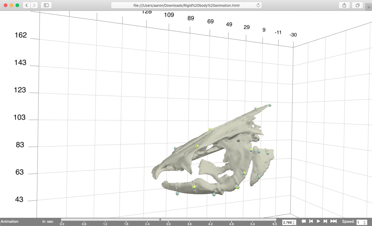
This should create the visualization shown below that can be opened in most major web browsers (currently works best in Chrome or Safari). Note that this is a standalone html file containing all of the code and mesh data needed for the visualization so it can be moved, e-mailed, etc. R is only needed to create the file, not to open it. The timeline along the bottom of the browser window has tools for controlling the animation playback, including the speed (far right). The animation is played back at realtime by default and this can be slowed down (<1) or sped up (>1) as needed.

From the animation you can see that the gray and yellow markers (the transformed landmarks and the motion capture coordinates, respectively) line up pretty well but not perfectly. This is what is expected when the unification errors are low because the two marker sets align well. Additionally, you'll notice how one skeletal element in particular, the suspensorium or "cheek bone" of the fish, is "wobbling". This is because all of the markers associated with that element are nearly co-linear and there is not enough information to fully "constrain" the motion of that element. Thus it tends to wobble about an axis defined by those nearly co-linear markers. We'll see further along in this tutorial how to reduce this wobble using "virtual points".

Using regular expressions in unify specifications

When we have lots of markers it gets a bit cumbersome to list the name of each marker in unify.spec. If the markers are labeled according to a consistent naming scheme then it's much simpler to use regular expressions. For example, the marker names in the tutorial dataset all begin with the body with which they're associated followed by an underscore and the word 'bead'. Thus, it's possible to re-write unify.spec as follows (since just a single regular expression is listed per body, the 'align' list can be omitted).

## Using regular expressions in unify specifications
# Specify which bodies to animate and which markers to use for each body
unify.spec <- list(
	'Neurocranium'='^Neurocranium_bead',
	'SuspensoriumL'='^SuspensoriumL_bead',
	'LowerJawL'='^LowerJawL_bead',
	'OperculumL'='^OperculumL_bead'
)

Then run unifyMotion with the regexp parameter set to TRUE (default is FALSE).

# Run unifyMotion with regexp to TRUE to use regular expressions in unify.spec
unify_motion <- unifyMotion(read_motion, xyz.mat=landmarks, unify.spec=unify.spec, 
	regexp=TRUE, plot.diag='Unify.pdf')

Saving the results for further analysis and export

There are a couple ways to save the results of unifyMotion. The first is to save the entire motion object using the writeMotion function. The motion object output by unifyMotion is exactly the same as the motion object that was put into the function only with the new body transformations added to it (as 'tmat'). It is best to save the whole motion object because this retains any metadata that have been added to the motion object (trial name, times, frame numbers, etc.).

## Saving the results
# Save motion
writeMotion(x=unify_motion$motion, file='Cat01 Trial09 body motion smoothed.csv')

This saved motion file can be then be read by using readMotion.

# Read saved motion
read_saved_motion <- readMotion(file='Cat01 Trial09 body motion smoothed.csv')

A second way to save the unification results is to just save the rigid body transformations. This is useful if you want to use the transformations in another program (such as to create an animation using Maya). To save only the rigid body transformations, use writeMotion but just including the 'tmat' object as shown below.

# Save just the transformations
writeMotion(x=list('tmat'=unify_motion$motion$tmat), file='Cat01 Trial09 body tmat smoothed.csv')

Lastly, since the unification errors are a matrix they can be saved simply by using the utils function write.csv function.

# Save the unification errors
write.csv(x=unify_motion$error, file='Unification errors.csv')

Visualizing motion relative to a particular body

When visually inspecting the results of unifyMotion it's often useful to fix the motion of one body. For example, with this tutorial dataset the catfish is swimming around the tank which makes it hard to see the motions of the skeletal elements in head. To get the motion of the elements relative to a particular body you can use the relativeMotion function. Input the motion object, which now includes the rigid body transformations, and the body that you would like to fix.

## Create animation of motion relative to neurocranium
# Get relative motion
relative_motion <- relativeMotion(motion=unify_motion$motion, fixed='Neurocranium')

The relativeMotion function outputs a new motion object in which all motions are relative to a fixed neurocranium. To create a new animation, simply re-run the code above but replacing the previous motion objects with relative_motion, as shown below.

# Create animation with fixed neurocranium
svg.new(paste0('Animation fixed Neurocranium.html'), mode='webgl')
for(body_name in names(unify.spec)){
	svg.mesh(paste0('meshes/Cat 01 ', body_name, '.obj'), name=body_name)
	markers_match <- grepl(paste0('^', body_name, '_'), dimnames(relative_motion$xyz)[[1]])
	body_markers <- dimnames(relative_motion$xyz)[[1]][markers_match]
	svg.spheres(relative_motion$xyz[body_markers,,], col='yellow')
}
svg.transform(relative_motion$tmat, times=relative_motion$time)
frame <- svg.frame()
svg.close()

Constraining body motion using "Virtual points"

You may have noticed (particularly in the preceding video with motion relative to the neurocranium) that the suspensorium or "cheek bone" of the fish, is "wobbling". This is because all of the markers associated with that element are nearly co-linear, causing the element to wobble about an axis defined by those nearly co-linear markers. To reduce this wobble we can add in extra landmarks (referred to as "virtual points" or "virtual markers") where we know that there is little motion of the element to help constrain the motion.

The suspensorium in catfish is attached to the neurocranium along a broad, hinge-like joint. One particular part of the joint has a tough ligament tethering the suspensorium to the neurocranium, preventing translation at that point and presenting an ideal virtual point to constrain the motion of the suspensorium (shown in the image below).

A virtual point (indicated by the red sphere) located at a ligamentous joint between the suspensorium and neurocranium can be added to supplement the markers and constrain the motion of the element. Click image to open interactive visualization.

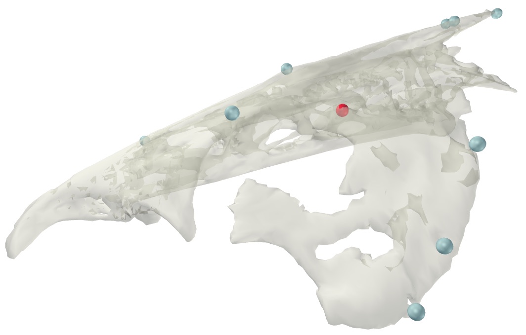
For the interested user, the visualization pictured above can be created using the following code:

## Constraining body motion using virtual points
# Create visual of virtual point
svg.new(paste0('Suspensorium virtual point.html'), mode='webgl')
for(body_name in c('Neurocranium', 'SuspensoriumL')){
	svg.mesh(paste0('meshes/Cat 01 ', body_name, '.obj'), opacity=0.5)
	markers_match <- grepl(paste0('^', body_name, '_'), dimnames(read_motion$xyz)[[1]])
	body_markers <- dimnames(read_motion$xyz)[[1]][markers_match]
	svg.spheres(landmarks[body_markers,], col='gray')
}
svg.spheres(landmarks['Neurocranium-SuspensoriumL_nc_susp_jt_cra',], col='red')
svg.close()

To use a virtual point during the unification step set the 3D coordinate of the virtual point (in the same coordinate system as the surface meshes) and add this to the marker landmarks file. I like to get virtual point coordinates in Blender by selecting a vertex on the mesh and then getting the vertex XYZ coordinate from the right-side panel (see below).

Blender can be used to get the 3D coordinate of a point on a mesh. The XYZ coordinate is shown near the top right corner under 'Transform'. Be sure that 'Local' is selected.

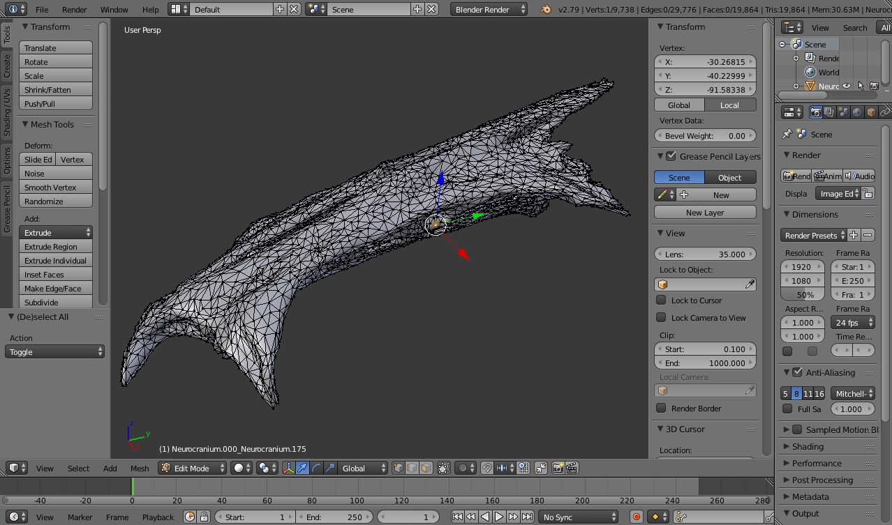
For the tutorial dataset this virtual point is labeled 'Neurocranium-SuspensoriumL_nc_susp_jt_cra' in the landmarks matrix. This virtual point will be animated with the neurocranium and then used to constrain the motion of the suspensorium.

To use the virtual point we just have to amend the unify.spec list. Under SuspensoriumL add a new list with two labeled items: 'align' and 'point'. The markers that will be used for the alignment (i.e. the markers we've been using so far) go under 'align' (this is the default). Then list any virtual points after 'point' in a named list, where the name of each virtual point group is the body used to animate the virtual point. In this case the name of the virtual point group is 'Neurocranium' since the virtual point is animated with the neurocranium.

# Add virtual point to unify specifications
unify.spec <- list(
	'Neurocranium'='^Neurocranium',
	'SuspensoriumL'=list(
		'align'='^SuspensoriumL',
		'point'=list('Neurocranium'='Neurocranium-SuspensoriumL_nc_susp_jt_cra')),
	'LowerJawL'='^LowerJawL',
	'OperculumL'='^OperculumL'
)

You can use as many virtual points as you'd like. For example, unify.spec for more than one virtual point animated with a body would be:

# Multiple virtual points
unify_spec2 <- list(
	'Body1'='^Body1',
	'Body2'=list(
		'align'='^Body2',
		'point'=list('Body1'=c('Body1VirtualPoint1', 'Body1VirtualPoint2')))
)

You can also use virtual points associated with multiple bodies. For example, unify.spec for multiple virtual points animated with multiple bodies would be as follows:

# Multiple virtual points
unify_spec3 <- list(
	'Body1'='^Body1',
	'Body2'='^Body2',
	'Body3'=list(
		'align'='^Body3',
		'point'=list(
			'Body1'=c('Body1VirtualPoint1', 'Body1VirtualPoint2')),
			'Body2'=c('Body2VirtualPoint1', 'Body2VirtualPoint2'))
)

If regexp is TRUE the virtual point names will be matched using regular expressions, just like the align points.

Importantly, unifyMotion does not treat virtual points in the same way as the markers or "align" points. Instead the function first finds the pose of the body using only the align points, an axis is fit to the align points at each iteration, and the body is rotated about this axis to minimize the distance between the virtual points animated with the parent body (here, the neurocranium) and the dependent body (here, the suspensorium). In this way the virtual points will not "pull" the body away from the markers but merely rotate the body around them. This has the effect of weighting the align markers more heavily than the virtual points (which is what we want since we know the align markers with more certainty than the virtual points). When the align markers are nearly co-linear a virtual point supplies additional information, based on known (anatomical) constraints, to constrain the motion about the axis with the most uncertainty while not compromising the reconstructed motion where there is more certainty. The unifyMotion function will automatically determine the order in which to solve for the body transformations given a particular hierarchy of virtual points so the order in which you list the bodies and virtual points in unify.spec doesn't matter.

After updating the unify specifications, call unifyMotion again.

# Unify motion using a virtual point
unify_motion <- unifyMotion(read_motion, xyz.mat=landmarks, unify.spec=unify.spec, 
	regexp=TRUE, plot.diag='Unify.pdf')

To visualize the results, create a new animation, adding a red sphere to indicate the new virtual point and reducing the opacity of the bones so that the virtual point is visible.

# Get motion relative to the neurocranium
relative_motion <- relativeMotion(unify_motion$motion, fixed='Neurocranium')

# Create an animation with the virtual point
svg.new(paste0('Animation virtual fixed Neurocranium.html'), mode='webgl')
for(body_name in names(unify.spec)){
	svg.mesh(paste0('meshes/Cat 01 ', body_name, '.obj'), name=body_name, opacity=0.7)
	markers_match <- grepl(paste0('^', body_name, '_'), dimnames(relative_motion$xyz)[[1]])
	body_markers <- dimnames(relative_motion$xyz)[[1]][markers_match]
	svg.spheres(relative_motion$xyz[body_markers,,], col='yellow')
}
svg.spheres(landmarks['Neurocranium-SuspensoriumL_nc_susp_jt_cra',], col='red', name='Neurocranium')
svg.transform(relative_motion$tmat, times=relative_motion$time)
frame <- svg.frame()
svg.close()

The addition of a single virtual point eliminates most of the previous wobbling.